Basic analysis of the trajectories

Overview

Teaching: 10 min
Exercises: 0 min

Questions

• Has my simulation converged?

• Is my protein stable?

Objectives

• Visualisation of MD trajectories.

• Basic analysis of MD trajectories.

Recentering the solutes in the simulation box

First of all, we need to recenter the protein to the center of the simulation box using cpptraj. cpptraj is the trajectory analysis tool of the AmberTools package and it can do a lot of different analysis (you can find more information here).

First, we need to load the topology file:

cpptraj -p system.parm7

Then, we provide cpptraj three different commands:

• trajin: input trajectories. It can be repeated as many times as trajectory file you want to analyse.
• trajout: output trajectories specifying the desired format.
• autoimage: recenters protein coordinates and fixes the simulation box around it.

After you have typed all your analysis commands you have to type go or run to actuallt make cpptraj run the analysis.

trajin system.md1.nc 1 100 10
trajin system.md2.nc 1 100 10
trajin system.md3.nc 1 100 10
trajin system.md4.nc 1 100 10 
trajin system.md5.nc 1 100 10
autoimage
center :1-305
trajout system.centered.nc netcdf
go 
quit

Visualise the shortened trajectory using VMD

To visualise the short trajectory you should type the following command:

vmd -m system.parm7 system.centered.nc

Some basic analysis of the simulation: RMSD and RMSF

Again, we will use cpptraj to analyse the trajectories. We will perform two very simple analysis:

Root Mean Square Deviation

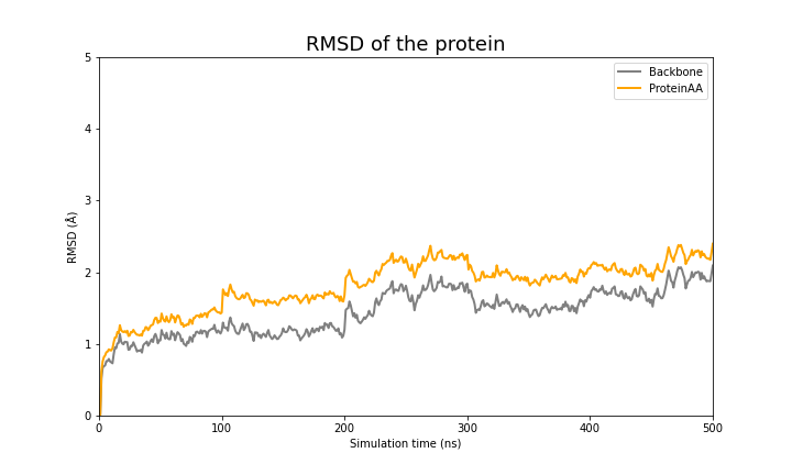
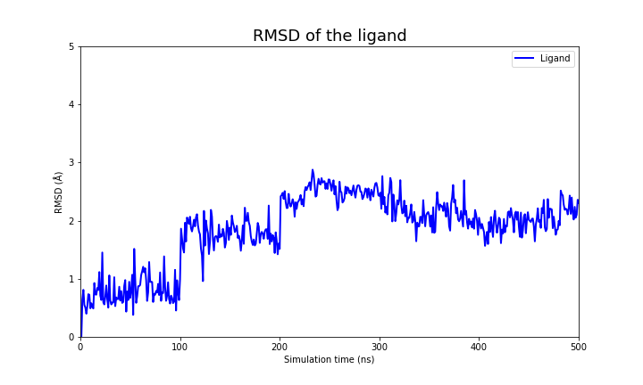
RMSD measures the deviation of a target set of coordinates (i.e. a structure) to a reference set of coordinates, with RMSD=0.0 indicating a perfect overlap. RMSD is defined as follows.

Root Mean Square Fluctuation

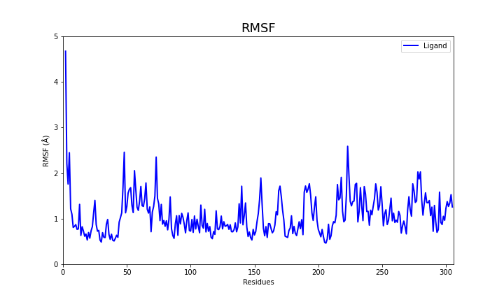
RMSF measures the deviation of each residue along the simulation time.

To perform the following analysis we will use all the frames of the trajectory and two new cpptraj commands: rms and atomicfluct.

Again to start the analysis, we start by loading the topology into cpptraj:

cpptraj -p system.parm7

Afterward we are going to use the following commands:

trajin system.md1.nc 
trajin system.md2.nc 
trajin system.md3.nc 
trajin system.md4.nc 
trajin system.md5.nc 
autoimage
center :1-305
rms fit :2-305@CA,C,N,O
rms ProtBB :2-305@CA,C,N,O first :2-305@CA,C,N,O out rmsd.txt mass fit
rms Ligand :1              first :1              out rmsd.txt mass nofit
rms ProtAA :2-305          first :2-305          out rmsd.txt mass nofit
atomicfluct Protein :2-305&!@H= byres out rmsf.txt 
go 
quit

As a result we obtain two files:

• rmsd.txt:
• rmsf.txt:

These two files if plotted show the following behavior:

RMSD

RMSD of the protein	Ligand

RMSF

Key Points

• It is important to recenter the protein to avoid analysis artefacts.

• It is ALWAYS good practice to visualise your simulations with VMD or Pymol.

• RMSD of the backbone a protein gives us a measure of its stability.